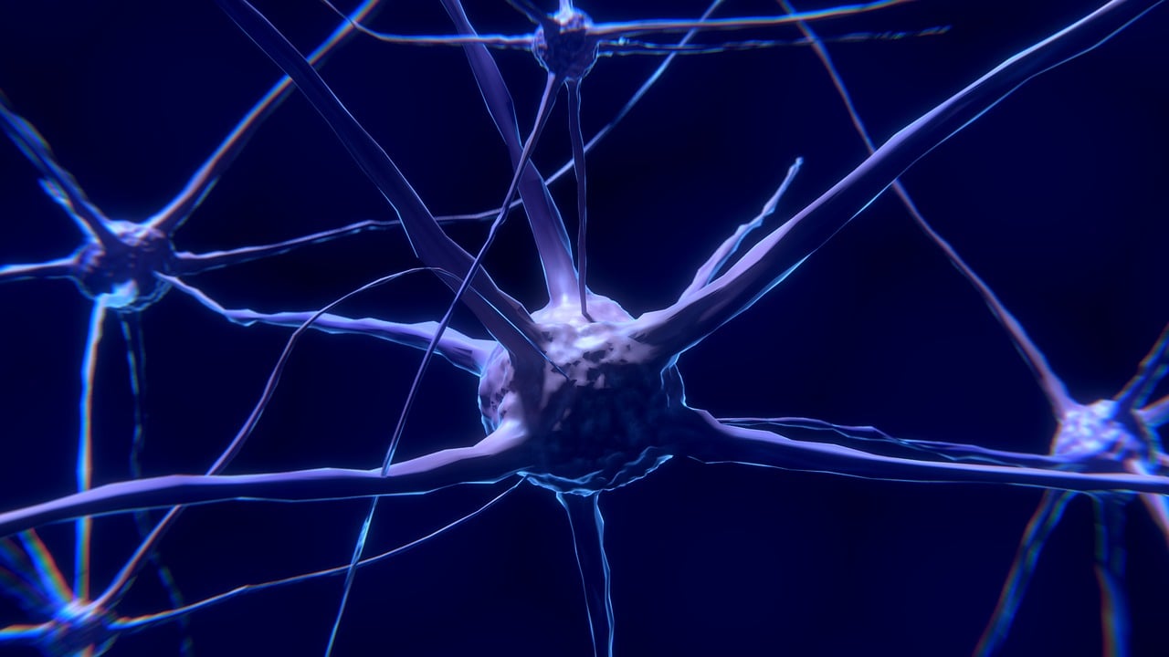
I heard about artificial neural networks first time around 2017. Since then I have tried to understand their behavior and explain them in a simple way.
Neural networks compared to traditional ML techniques
Neural networks are very adaptible systems. In practice this means that they can learn complex patterns without explicit definition. It has been said, that feature engineering can be totally skipped.
Many neural networks architectures can be trained efficiently to make predictions for unseen scenarios.
Both of these arguments apply to common definition of machine learning. Neural networks just take these aspects further. As a downside neural network internal behavior is not as easy to explain than the traditional ML models.
Data for neural network example
Example case: Predict loan risk by applicant age. The training data could be something like this. Neural networks work better with normalized values, so the age is scaled between 0 and 1. One row is one person.
| age_years | age_scaled | risk |
|---|---|---|
| 20 | 0.0 | 0.8 |
| 40 | 0.5 | 0.1 |
| 60 | 1.0 | 0.3 |
| … | … | … |
The aim is to predict credit risk by the age_scaled.
Neural network with 1 input and 1 output
The simplest possible neural network architecture looks like this:
O - O
It has input node O, one edge - and output node O.
Each observation in the training set runs through this “network”.
The first observation in the loan data had age of 0.0. That is the input. Simple math is applied at the output node to get a prediction for the 20-year old:
ActivationFunction(0.0*[Weight]+[Bias]) = [Predicted Risk]
This simple formula is the foundational for neural networks. But the activation function, weight and bias require a bit more explanation.
Neural network with multiple inputs and 1 output
Let’s take a step further. This could be a neural network that predicts loan risk by applicant age, income and shoe size. Three inputs and one output. The smart guys would call it as multivariate regression. Or just linear regression with three variables…
O \
O - O
O /
Math is not yet too complex after the first iteration:
[Predicted Risk] = ActivationFunction(20*[Weight 1]+[Bias]+20*[Weight 2]+20*[Weight 3]+[Bias])
Weight and bias in neural networks
Each edge in neural network has a weight. They are initialized randomly.
And each node has bias. It is a node specific constant value added to the calculation.
The generic formula for a node values is:
ActivationFunction([Input 1]*[Weight 1]+[Input 2]*[Weight 2]+[Input n]*[Weight n]+[Bias])
Activation function
Activation function sounds scary, but the math is rudimentary.
Simplest activation function might be a linear one. It keeps the value the same than it was.
Maybe more common one is ReLU. Despite of the weird name it just converts negative values to zero. In the end, it does not make sense to mix positive and negative value to plus calculation that are in the core of the neural network. Large positive and large negative would become close to zero.
Here is a summary table of common activation functions:
| Neural network activation function | How it works | When to use |
|---|---|---|
| Linear | No conversion | |
| ReLU | Convert negative to zero, otherwise value remains. | Deep networks. |
| Leaky ReLU | Negative values are just slightly negative. | To avoid vanishing gradients |
| Sigmoid | Probabilities [0, 1] for two-class classification. The name referes to S-shape by definition. | Output layer. Logistic regression. |
| Softmax | Probabilities [0, 1] for multi-class classification | Output layer. |
| TanH | Like sigmoid but can result values [-1, 1]. | RNN and NLP. |
Sigmoid and TanH should no be used with deep networks due to vanishing gradients.
Neural network loss
Each observation runs through the network. Whatever weights the edges might have are applied to in the activation functions. Well, in the simple example there was only one activation that happened in the output node.
Loss is the prediction error in the output.
Let’s say that the we used a linear activation function (no conversion) and the value in output node was 0.32. This is our prediction. The actual value was 0.8. If our loss metric is mean absolute error the total loss would be simply:
0.8 - 0.32 = 0.48
After running each iteration the loss metric is calculated again. By plotting these values we can create a loss curve to visuzlize progress. Loss curve should decrease exponentially.
Here are some common neural network loss functions:
| Neural network loss function | Explanation |
|---|---|
| Mean Average Error | Simple. |
| Means Squared Error | Emphasizes big errors. |
Updating weights by backpropagation and gradient descent
A neural network is just a bunch of simple mathematical calculations. Having enough of them makes the model complex.
Gradient descent is the algorithm that calculates the new edge weights after each observation has ran through the network.
As you see, this situation could be identical to a univariate linear or logistic regression depending on the activation function.
There are two fundamental parameters for gradient descent: Step size and step direction. The step size is known as learning rate of the model.
Here are the trade-offs for learning rate:
| Gradient descent step size | Problems |
|---|---|
| Too small | Training takes long time. Might get stuck to local optima. |
| Too big | Loss curve starts oscillating and does not converge. |
Neural network otimizers
Optimizer are variants of gradient descent algorithm. The aim for optimzing the step size or direction to train optimal model as quickly as possible.
| Neural network optimizer | Full name | When to use |
|---|---|---|
| SGD | Stochastic Gradient Descent | Common default. |
| Adam | Adaptive Moment Estimation | Large dataset, lots of parameters. |
| Adamgrad | Adaptive Gradient Optimizer | Adjust step size per feature. |
Neural network mini-batches
Running gradient descent in mini batches reduces the loss graph variation and makes it more readable. This means that loss calculation and weight update is done only after multiple observations.
Some sources recommend 10-1000 observations per mini-batch, some 40-100. If there are too many, the iteration does not fit into computer memory. Also, you the program crashing after long period of time would more costly.
Mini-batches also allow program to run similar operation in parallel which a huge performance boost.
Larger batch sizes require smaller learning rates.
Epochs in neural network training
Epoch means running the whole dataset through the neural network. A typical training consists of multiple epochs.
Virtual epochs can be used for large and varying amounts of data. With this approach, epoch can be any size, not necessarily the whole dataset.
Monitoring training issues
Common problematic behavior that can be detected from loss curve:
| Loss curve behavior | Explanation |
|---|---|
| Oscillating | Learning rate too big |
| Converges slowly | Learning rate too small |
| Diverges (goes up) | Overfitting, try simpler model. |
| Not converging | Underfitting, try more complex model. |
| Increases sharply | Anomalous values that cause NaN traps or exploding gradients. |
Number of layers in neural network
More hidden layers can learn more complex non-linear patterns.
A layer can be thought as a step in feature engineering. The model is doing some of that work automatically!
Neural network with multiple inputs and multiple outputs
In this example input features are risk applicant’s age, income and shoe size. On top of the loan risk level the model predicts also loan repayment time and customer lifetime value.
Multiple multivariate regressions at once. This would correspond having three linear regressions that are somewhat tied together.
This graph tries to present that connections go from each input to each output. 9 edges in total.
O <- O
O <- O
O <- O
Neural network with multiple inputs, multiple outputs and a hidden layer
Inputs and output could again be the same as above. But we also have a hidden layer with 3 nodes. Now 18 edges in total.
The hidden layer is not controlled. The nodes do not have explanation that directly connects to real world. It is just a vector of three items.
But you can think that the middle step would describe the applicant by three attributes: Population of the city they live in, reliability of their workplace and person’s cost awareness.
Or maybe this would correspond running principal component analysis before training. In PCA, synthetic features are created to reduce dimensionality.
O <- O <- O
O <- O <- O
O <- O <- O
A neural network with multiple hidden layers can be called deep. Deep neural networks are performing well with highly correlated features compared to linear models.
Linear vs non-linear network
According to discussion, multiple linear layers in neural network will not make it non-linear.
To achieve model non-linearity, non-linear activation functions such as ReLU, sigmoid or tanH must be used.
Google materials state that non-linearity speeds up training and improves accuracy without loss of important information.
Neural network architectures
Here are some neural network models you might read about in the internet:
| Neural network architecture | Use case |
|---|---|
| ANN | Artificial Neural Network. The umbrella term. |
| DNN | Deep Neural Network. A network with hidden layers. |
| GAN | Generative Adversial Networks. Tries to reproduce samples (images). |
| CNN | Convolutional Neural Network. Image classification. Pixel relationships matters a lot. |
| RNN | Recurrent Neural Network. A network that has memory of previous step. Suitable for NLP and time series. |
| LSTM | Long Short-Term Memory. Time series forecasting. |
| GRU | Gated Recurrent Unit. LSTM with forget unit, fewer parameters and no output. |
| Resnet | Deep Residual Learning for image recognition to tackle vanishing gradients. |
| Autoencoder and self-encoder | Create embeddings in a hidden layer by |
| TabNet | Deep network to with sequential attention using the best features on each step. |
| AdaNet | Adaptive neural network that tries various sub networks. |
| DCN | Deep & Cross Network for recommenders. |
| R-CNN | Regional CNN. Identify multiple objects from image by splitting to 2000 regions. |


Write a new comment
The name will be visible. Email will not be published. More about privacy.